
Introduction
GALEXSpec is an IDL program for examining GALEX spectra. It is not an “official” GALEX product, but I will nevertheless do my best to support and improve the program. As explained in more detail in the GALEX Spectroscopy Primer, the GALEX spectra are a challenge to extract from the raw data, largely because the data are obtained without slits and the overlapping spectra must be disentangled using many rotations of the grism. GALEXSpec is a handy program for stepping through all the spectra obtained in a field and includes tools for assessing how a particular spectrum has been disentangled from its neighbors. You might also find the gallery of GALEX spectra useful.
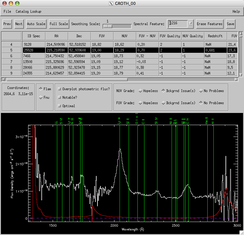
Figure 1. A screen shot of the main window of the GALEXSpec program showing a z = 0.681 quasar in the GROTH_00 field.
Obtaining the Code
The program is written in IDL and requires IDL 6.0 or later. The code can be downloaded using the links on the left, or, most speedily, using the link immediately below. You need to download the files (currently version v0.4.8 beta):
You will also need the IDL Astronomy User's Library and David Fanning's Coyote Program Library. Both of these libraries are free.
Compiling the Code
Compiling the code is a little tedious since, because I insist on using mixed case file names, the three files must each be compiled twice. With newer versions of IDL (6.4 and above) this may not be necessary.
Box 1. The commands for compiling the three files that comprise GALEXSpec. (Yes, you need to type each command twice).
Using the Program
The extracted 1D spectra are contained in the -xg-gsp.fits files. In addition, the program uses the -ng-pr[c|i].fits and -fg-pr[c|i].fits files (which contain the 2D spectral image strips), the -ng-gsax.fits and -fg-gsax.fits files (which contain additional information about the spectra), and optionally the -nd-int.fits and -nd-int.fits files (which contain the direct images). The program is started using the command RunGALEXSpec. RunGALEXSpec accepts the following keywords:
- autoSave -- should the contents of the GALEXSpec table automatically saved every five minutes?
- browser -- the path to the executable for your favorite web browser. The defaults are Safari on Mac OS X and Firefox on Linux.
- fuvLimit -- objects fainter than fuvLimit will not be displayed.
- grismPath -- the path to the directory containing the grism data.
- imagePath -- the path to the directory containing the imaging data.
- inputTable -- if you've previously run GALEXSpec on these data and saved the table, you can restart GALEXSpec with the old input table.
- noStamp -- set this keyword to not display the postage stamp images.
- nuvLimit -- objects fainter than nuvLimit will not be displayed.
- radiusLimit -- objects with radii larger than this limit will not be displayed.
- soda -- set this keyword if your data are stored on disk in the same layout as the GALEX SODA layout, or set to a string containing the path to the top level SODA tile directory.
- visit -- set this keyword to indicate that the data are single visit (as opposed to co-added “main”) data. If you also set the soda keyword, you can set this to a specific visit number.
- nuvOnly -- set this keyword if there are no FUV grism data.
If you specify paths to the data using some combination of the grismPath, imagePath, and soda keywords, then the program will pop up one (only use grism data with the noStamp flag set) or two (use both grism and imaging data) file selection windows for you to use.
If all goes well, you should eventually see three IDL widget windows open on your display: the main window with lots of buttons, a table with an entry for each spectrum, and a plot window (Figure 1); the image strips window displaying the two-dimensional image strips for both bands (Figure 2); and the postage stamps window showing the direct images of the object (Figure 3).
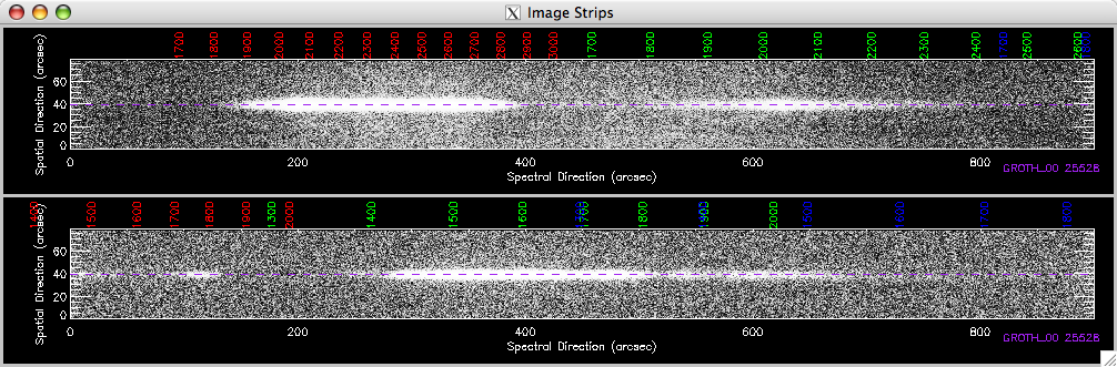
Figure 2. A screen shot of the image strips window of the GALEXSpec program showing a z = 0.681 quasar in the GROTH_00 field.
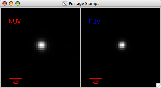
Figure 3. A screen shot of the postage stamps window of the GALEXSpec program showing a z = 0.681 quasar in the GROTH_00 field.
The "File" menu contains five options:
- Open a new tile.
- Create a Postscript version of the spectrum. (Example)
- Create a three-column ASCII file containing the wavelength, flux, and error. (Example)
- Create a Postscript screen shot of all of the GALEXSpec windows. Apple's Preview program doesn't convert the Postscript into PDF well (in fact, you won't see anything). However, both gv and Adobe Distiller will deal with the files just fine. (Example)
- Create a FITS binary table containing the wavelength, flux, and error data for the spectrum. (Use right-click and "Save Link As" to download Example)
- Quit the program.
The "Catalog Lookup" menu allows you to look up an object (by position) in the SDSS or NED databases.
The "Help" menu contains two items:
- About gives the current version and a cheat sheet for the keyboard commands.
- Keystrokes and Mouse info prints the cheat sheet to your terminal.
Buttons, sliders, and so on:
- Prev -- moves backwards in the table of spectra.
- Next -- moves forwards in the table of spectra.
- Autoscale -- autoscales the y-axis of the current spectrum.
- Full Scale -- scales the y-axis to the full range of flux values in the current spectrum.
- Smoothing Scale -- boxcar smoothing length (usually left at 1).
- Spectral Feature -- the rest wavelength of the spectral feature to be marked. There is a default list of features and additional features can be added by hand. (See the mouse commands below.)
- Erase Features -- erase features previously marked.
- Save -- save the table as a FITS binary file, which can be reloaded into GALEXSpec.
The table widget lists all the extracted spectra in the field (modulu the magnitude and radius limits). The quantities listed in the table are the following:
- ID Spec -- the ID of the spectrum.
- RA -- right ascension.
- Dec -- declination.
- FUV -- FUV magnitude from direct imaging.
- NUV -- NUV magnitude from direct imaging.
- FUV - NUV -- Color from direct imaging.
- FUV Quality -- An automatic assessment of the quality of the spectrum. See the GALEX Spectroscopy Primer for details. The quality can be changed using the toggle switches in the Grades area.
- NUV Quality -- An automatic assessment of the quality of the spectrum.
- Redshift -- the redshift of the object. This will be NaN unless you've measured the redshift.
- FUV SNR -- the median FUV signal-to-noise ratio computed using the error spectrum.
- NUV SNR -- the median NUV signal-to-noise ratio computed using the error spectrum.
- FUV FWHM -- the FWHM of the FUV image of the source (arcseconds).
- NUV FWHM -- the FWHM of the NUV image of the soruce (arcseconds).
- Radius -- the radius of the source from the field center (degrees).
- GGOID -- the GALEX global object ID. A 64 bit number displayed as two 32-bit numbers.
- Notable -- a flag to mark interesting objects.
The miscellaneous region below the table contains a read out of the coordinates (wavelength in Angstroms and flux in cgs units), a toggle to switch between Flambda and Fnu, a button to overplot the source flux measured in the images, a button to toggle the notability status, and a series of buttons to manually adjust the grade or quality of the spectrum.
Plot Window (Figure 1). By default, the plot window shows the spectrum with the flux axis autoscaled. The spectrum is shown in white with the 1 sigma error spectrum shown in red. The dashed purple line marks zero flux. You can zoom in by holding down the left mouse button and drawing a box to mark the desired axis ranges. A spectral feature can be marked (and thus the redshift calculated) using the right mouse button. All features in the features database will be marked and labelled in green.
The plot window contains a few keyboard shortcuts:
- a -- autoscale the spectrum.
- b -- plot the background.
- f -- full scale the spectrum.
- n -- next spectrum.
- p -- previous spectrum.
- r -- redraw the spectrum.
- y -- spatial profile of the spectrum.
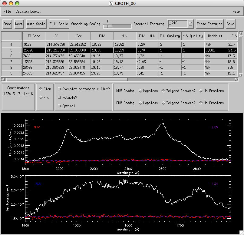
Figure 4. The background panels (NUV top, FUV bottom) show the uncalibrated source flux (white) and the background (red).
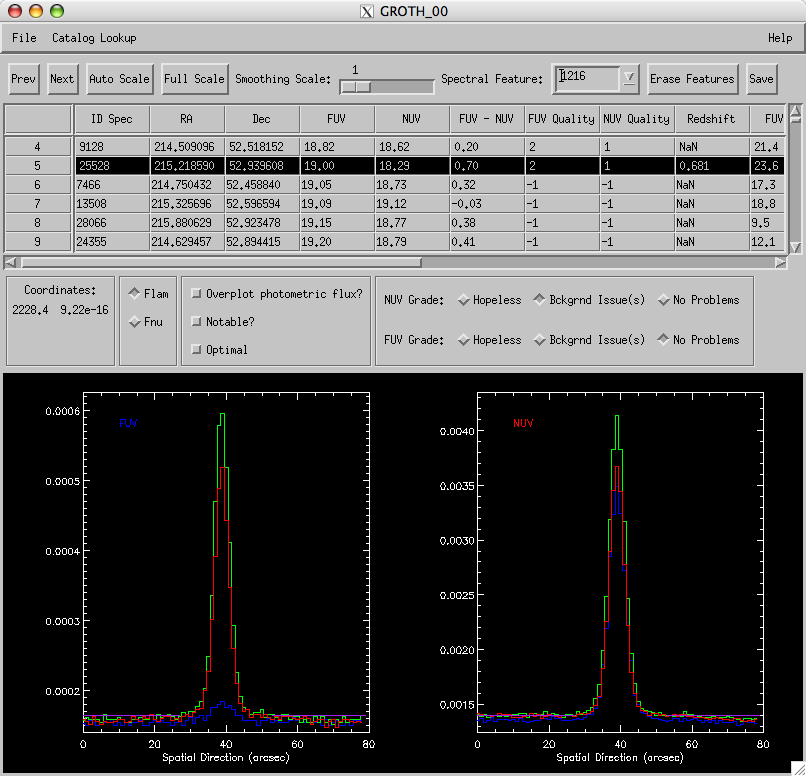
Figure 5. The profile panels show the spatial profiles (i.e, a cut along the spatial direction) for the short (blue), middle (green), and long (red) wavelength sections of the FUV (left) and NUV (right) spectra. The purple lines mark the regions from which the background is extracted.
Image Strips (Figure 2). The image strips window shows the NUV (top) and FUV (bottom) 2D image strips. Since there is no order blocking filters, multiple orders are often visible. The wavelengths for the 1st, 2nd, and 3rd orders are labelled in red, green, and blue, respectively. By default, the strips are displayed with histogram equalization. However, a linear stretch can be applied by left-clicking in either window and dragging. Pressing "h" will return to histogram equalivation.
Postage Stamps (Figure 3). The postage stamp windows show the images of the objects with a linear stretch. The stretch can be adjusted by left-clicking and dragging. Pressing "h" will switch to histogram equalivation.
FAQ
The program has crashed, leaving abandoned widgets and huge memory leaks. What do I do?
Box 2. If the program crashes, which, alas, it will, these three IDL commands will be your friends.
What do the FUV and NUV quality numbers mean?
The quality numbers are explained in detail in the GALEX Spectroscopy Primer, but the gist is: 0 = hopeless, 1 = a significant background issue is marring the spectrum, 2 = okay.
What do the numbers in purple in the upper right of the background panels mean?
The little purple numbers are a measure of the ratio of the large scale (low frequency) background fluctuations to the small scall (high frequency) background fluctuations. Spectra are automatically flagged as having background issues if this number is greater than 1.5 for NUV and 1.3 for FUV.
Feedback
Please let me know if you have any comments, questions, or suggestions.